Lesson 07: Modeling Digital Circuits in Verilog
Verilog HDL provides three levels of abstraction for describing digital circuits: gate-level, dataflow, and behavioral modeling. Each modeling style serves different purposes and offers varying levels of detail and ease of use.
7.1 Gate-Level (Structural) Modeling
Gate-Level Modeling
Gate-level modeling (also known as Structural Modeling) can be used to write Verilog codes for small designs. Verilog HDL supports built-in primitive gates modeling. The gates supported are multiple-input, multiple-output, tristate, and pull gates. The multiple-input gates supported are: and, nand, or, nor, xor, and xnor, whose number of inputs is two or more and has only one output. The multiple-output gates supported are buf and not whose number of output is one or more and has only one input. The language also supports tri-state gates modeling, including bufif0, bufif1, notif0, and notif1. These gates have one input, one output, and one control signal. The pull gates supported are pullup and pulldown with only a single output (no input).
Steps for Gate-Level Modeling:
- Define the Module: Declare the module and its ports.
- Instantiate Gates: Use predefined gate primitives (e.g., and, or, not) or user-defined gate modules.
- Connect Gates: Connect the gates using wires.
For gate-level modeling, the combinational logic circuit schematic must be drawn first.

Figure 1: Schematic
The first step in gate-level modeling is to check that all wires must have unique names. All the input/output wires have the same name as the I/O port name. In the Circuit Diagram of Figure 1, the output wires of the NOT and AND gates have no name, and they should be assigned a name. The wire name nc indicates the output wire of the NOT gate, and y0 indicates the output of the AND gate.
In the second step, use logic gates to describe the schematic from left to right, top to bottom.
Based on the schematic shown in Figure 1, the Verilog code can be written as follows:
module circuit1(a, b, c, f);
    input  a, b, c;
    output f;

    wire  nc, y0;

    not U1 (nc, c);
    and U2 (y0, b, nc);
    or  U3 (f, y0, a);

endmodule
In the gate-level modeling, only the gates and wires can be used in the code.
Gates
The gates have one scalar output and multiple scalar inputs. The first terminal in the list of gate terminals is an output, and the other terminals are inputs.
The basic syntax for each type of gate with zero delays is as follows:
and | nand | or | nor | xor | xnor [instance name] (out, in1, …, inN); // [] is optional and | is selection

| Gate | Description | Syntax |
| or | N-input OR gate | or GateName(out, in1, in2, in3, ...); |
| and | N-input AND gate | and GateName(out, in1, in2, in3, ...); |
| xor | N-input XOR gate | or GateName(out, in1, in2, in3, ...); |
| nor | N-input NOR gate | nor GateName(out, in1, in2, in3, ...); |
| nand | N-input NAND gate | nand GateName(out, in1, in2, in3, ...); |
| xnor | N-input XNOR gate | xnor GateName(out, in1, in2, in3, ...); |
Buffer and NOT Gates
The basic syntax for each type of gate with zero delays is as follows:
buf | not [instance name] (out1, out2, …, out2, input);

| Gate | Description | Syntax |
| buf | N-output buffer | buf GateName(out1, out2, ..., in); |
| not | N-output NOT gate | not GateName(out1, out2, ..., in); |
Tri-State Gates
The basic syntax for each type of gate with zero delays is as follows:
bufif0 | bufif1 | notif0 | notif1 [instance name] (outputA, inputB, controlC);

| Gate | Description | Syntax |
| bufif0 | Tri-state buffer with active-low control | bufif0 GateName(out, in, ctrl); |
| bufif1 | Tri-state buffer with active-high control | bufif1 GateName(out, in, ctrl); |
| notif0 | Tri-state NOT gate with active-low control | notif0 GateName(out, in, ctrl); |
| notif1 | Tri-state NOT gate with active-high control | notif1 GateName(out, in, ctrl); |
Pullup and Pulldown for Output Pins
The basic syntax for each type of gate with zero delays is as follows:
pullup | pulldown [instance name] (output A);
Gate-level modeling is useful when a circuit is a simple combinational circuit, such as a multiplexer. A multiplexer is a simple circuit that connects one of many inputs to an output. In this part, you will create a simple 2-to-1 multiplexer and extend the design to multiple bits.
Gate-Level Modeling of a 4x1 Multiplexer
Using gate-level modeling, write a Verilog description of the 2-to-4 decoder as shown below.

module mux_4to1(in0, in1, in2, in3, s0, s1, out);
    input  in0, in1, in2, in3, s0, s1
    output out;

    wire ns0, ns1;
    wire a0, a1, a2, a3;

    not N0 (ns0, s0);
    not N1 (ns1, s1);
    and G0 (a0, ns0, ns1, in0);
    and G1 (a1, ns0,  s1, in1);
    and G2 (a2,  s0, ns1, in2);
    and G3 (a3,  s0,  s1, in3);
    or  G4 (out, a0, a1, a2, a3);

endmodule
Questions
Gate-level (structural) modeling will be used to solve the following questions.
- Using gate-level modeling, write the Verilog module to implement the circuit in the following figure.
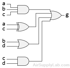
- Write a Verilog description to implement the circuit shown in the figure using gate-level modeling.

7.2 Dataflow Modeling
Gate-level modeling is useful for writing Verilog code for small designs. However, using gate-level modeling to write Verilog code for large designs may be cumbersome. Dataflow modeling can be used to describe the behavior of large circuits. This type of modeling uses Boolean operators and logical expressions. Hence, dataflow modeling in Verilog allows a digital system to be designed in terms of function.
Dataflow modeling uses Boolean equations and many operators that operate on inputs to produce outputs. There are approximately 30 Verilog operators. These operators can be used to synthesize digital circuits. Some of the operators are listed in the Lesson 05: Operands, Expressions, and Operators
Dataflow modeling uses continuous assignments and the keyword "assign". A continuous assignment is a statement that assigns a value to a net. The net data type in Verilog HDL represents a physical connection between circuit elements. The value assigned to the net is specified by an expression that uses operands and operators. This style is often used to describe combinational logic and is more abstract than gate-level (structural) modeling.
Key Concepts in Dataflow Modeling:
- Continuous Assignment: The core of dataflow modeling is the continuous assignment statement (assign). It is used to drive values onto nets.
- Operators: Various operators (arithmetic, logical, bitwise, and reduction) are used to describe data transformations and data flow.
- Nets: Typically, dataflow modeling uses a wire type to represent connections between different parts of the design.
Syntax of Continuous Assignment:
assign <net> = <expression>;
- net: The net to which the result of the expression is assigned.
- expression: The combination of signals and operators that defines the desired logic.
Examples:
Example 1: Simple AND Gate
Let's start with a simple AND gate using dataflow modeling.
assign y = a & b;
Example 2: 1-bit 2-to-1 MUX
As an example, assuming that the variables were declared, a 1-bit 2-to-1 multiplexer with data inputs a and b, select input s, and output y is described with a continuous assignment:
assign y = (a & s) | (b & s);
// or
assign y = (s) ? b : a;
Example 3: 1-bit Half Adder
A 1-bit half-adder using dataflow modeling.
assign {carry_out, sum} = a + b;
7.3 Behavioral Modeling
Behavioral modeling in Verilog describes a digital circuit using logic expressions and C-like constructs. Behavioral modeling allows a designer to describe circuits based on their function rather than their gate-level structure. Usually, it describes how outputs are computed from inputs and how internal states change under specific conditions.
Key concepts in behavioral modeling include:
- Always Blocks: Used to describe behavior triggered by signal changes or clock edges.
- Procedural Statements: Include constructs like if, case, for, while, repeat, and forever.
- Registers: Variables of type reg are commonly used in procedural descriptions.
- Sensitivity List: Determines when an always block executes.
In behavioral modeling, assignments are not carried out continuously. Instead, they occur in response to events specified in the sensitivity list. This modeling style is implemented using procedural blocks. All procedures in Verilog are specified within one of the following four constructs:
- always block
- initial block
- task
- function
Tasks and functions are additional procedural constructs that are activated by other procedures. Their detailed usage will be introduced in a later lesson dedicated to reusable procedural coding techniques."Lesson 15: Tasks, Functions, and Directives".
The initial and always statements are enabled at the beginning of the simulation. The initial statement executes only once, while the always statement executes repeatedly until the simulation ends. They are comparable to the setup() and loop() functions in Arduino C. There is no limit to the number of initial and always blocks that can be defined in a module.
Also, the output variables must be declared reg because they must retain their previous value until a new assignment occurs after any change to the specified sensitivity list.
initial Procedure
An "initial" statement is executed only once in the simulation.
The syntax for the initial block is as follows:
initial [timing_control] procedural_statement;
initial [timing_control] begin
multiple_procedural_statements;
end
The initial statement is non-synthesizable and is normally used in test benches to generate inputs at the desired time to test the module.
always procedure
Each "always" statement repeats continuously throughout the simulation run and circuit execution.
The syntax for the always block is as follows:
always @ (<sensitive List>) procedural_statement;
always @ (<sensitive List>) begin
multiple_procedural_statements;
end
The always statement is synthesizable, and the resulting circuit can be combinational or sequential.
For the model to generate a combinational circuit, the always block must meet all the following requirements:
- It should not be edge-sensitive.
- Every branch of the conditional statement should define all outputs.
- Every case statement should define all outputs and include a default case.
To generate a sequential circuit, the always block must meet the following requirements:
- It should be edge-sensitive, such as posedge clk or negedge clk.
- It should use non-blocking assignment <= to model register behavior correctly.
Procedural Assignments
Procedural assignments are used in Verilog's always and initial blocks to describe the behavior of a digital system. They allow you to model complex logic and control structures. Procedural assignments can be classified into blocking and non-blocking assignments, each serving a different purpose and having distinct characteristics.
Types of Procedural Assignments:
- Blocking Assignments (=)
- Non-Blocking Assignments (<=)
Blocking Assignments (=)
Blocking Assignments (=)
Blocking assignments are executed sequentially, blocking execution of the next statement until the current one completes. They are typically used for combinational logic.
Syntax
always @ (sensitivity list) begin
    reg_variable = expression;
    // Other sequential statements
endExample: Combinational Logic using Blocking Assignments
module blocking_example ( a, b, y);
    input  a, b;
    output y;

    reg y;

    always @(*) begin
        y = a & b;  // Blocking assignment
    end

endmodule
Non-Blocking Assignments (<=)
Non-Blocking Assignments (<=)
Non-blocking assignments are executed concurrently, allowing the next statement to execute without waiting for the current one to complete. They are typically used for sequential logic and register updates.
Syntax
always @ (posedge clk or posedge rst) begin
    if (rst)
        reg_variable <= reset_value;
    else
        reg_variable <= expression;
    // Other sequential statements
endExample: Sequential Logic using Non-Blocking Assignments
module nonblocking_example ( clk, rst, d, q);
    input  clk, rst, d;
    output q;

    reg q;
    always @(posedge clk or posedge rst) begin
        if (rst)
            q <= 1'b0;  // Non-blocking assignment
        else
        q <= d;
    end

endmodule
Common Pitfalls and Best Practices:
- Use Non-Blocking Assignments for Sequential Logic: Always use non-blocking assignments (<=) for registers in sequential logic to avoid race conditions and ensure proper timing.
- Use Blocking Assignments for Combinational Logic: Use blocking assignments (=) for combinational logic to ensure correct evaluation order within the always block.
- Avoid Mixing Assignments: Do not mix blocking and non-blocking assignments for the same variable within the same always block. This can lead to unpredictable behavior.
- Complete Sensitivity Lists: Ensure that the sensitivity list in combinational always blocks includes all relevant signals to avoid simulation mismatches.
- Test Thoroughly: Use test benches to simulate and verify your design's behavior. This helps catch procedural assignment issues early in the design process.
Example 1: Simple Sequential Logic (D Flip-Flop)
Define the Module:
module d_flip_flop ( clk, rst, d, q);
    input  clk, rst, d;
    output q;

    reg q;

    // Always block for sequential logic
    always @(posedge clk or posedge rst) begin
        if (rst)
            q <= 1'b0; // Reset condition
        else
            q <= d; // On clock edge, q takes the value of d
    end

endmodule
Explanation
- Module Definition: The d_flip_flop module has inputs clk, rst, and d, and an output q.
- Register Declaration: q is declared as reg because it stores the value.
- Always Block: Triggered on the rising edge of clk or the rising edge of rst.
- Procedural Statements: if-else statement checks the reset condition. If rst is high, q is set to 0. Otherwise, q is assigned the value of d on the clock edge.
Example 2: 4-bit Counter with Enable
Define the Module:
module counter ( clk, nrst, en, count);
    input  clk, rst, en;
    output [3:0] count;

    reg [3:0] count

    // Always block for sequential logic
    always @(posedge clk or negedge rst) begin
        if (!rst)
            count <= 4'b0000;  // Reset count to 0
        else if (en)
            count <= count + 1;  // Increment count if enabled
    end

endmodule
Explanation
- Module Definition: The counter module has inputs clk, nrst, and en, and an output count.
- Register Declaration: count is a 4-bit register.
- Always Block: Triggered on the rising edge of clk or the falling edge of nrst.
- Procedural Statements: if-else statement checks the reset condition and enables the signal. If nrst is low, the count is reset. If en is high, count is incremented.
Example 3: 8-bit Equality Comparator
Define the Module
module comparator ( a, b, eq);
    input  [7:0] a;
    input  [7:0] b;
    output       eq;

    reg eq;
    // Always block for combinational logic
    always @(*) begin
        if (a == b)
            eq = 1'b1;
        else
            eq = 1'b0;
    end

endmoduleExplanation:
- Module Definition: The comparator module has inputs a and b, and an output eq.
- Register Declaration: eq is declared as reg because it is assigned within an always block.
- Always Block: Triggered whenever there is a change in a or b (combinational logic).
- Procedural Statements: if-else statement checks if a is equal to b and sets eq accordingly.
Example 4: Traffic Light Controller (Finite State Machine)
Define the Module:
module traffic_light_controller ( clk, nrst, lights);
  input        clk, nrst;
  output [1:0] lights;

    reg [1:0] lights;

    // State encoding
    typedef enum reg [1:0] {S_RED, S_GREEN, S_YELLOW} state_t;
    state_t curr_state, next_state;

    // State transition logic
    always @(posedge clk or negedge rst) begin
        if (!rst)
            curr_state<= RED;
        else
            curr_state<= next_state;
    end

    // Next state logic
    always @(*) begin
        case (state)
            S_RED:
                next_state = GREEN;
            S_GREEN:
                next_state = YELLOW;
            S_YELLOW:
                next_state = RED;
            default:
                next_state = RED;
        endcase
    end

    // Output logic
    always @(*) begin
        case (curr_state)
            S_RED:
                lights = 2'b00;
            S_GREEN:
                lights = 2'b01;
            S_YELLOW:
                lights = 2'b10;
            default:
                lights = 2'b00;
    endcase
  end

endmodule
Example Testbench for the Traffic Light Controller:
`timescale 1ns/1ps
module traffic_light_controller_tb;
    reg clk;
    reg nrst;
    wire [1:0] lights;

    // Instantiate the traffic_light_controller
    traffic_light_controller UUT (
        .clk(clk),
        .nrst(nrst),
        .lights(lights)
    );

    // Clock generation
    initial begin
        clk = 0;
        forever #5 clk = ~clk;  // 10 time units clock period
    end

    // Test sequence
    initial begin
        // Initialize signals
        nrst = 0;
        #10 nrst = 1;  // Release reset after 10 time units

        // Observe the output
        #100;  // Run simulation for 100 time units
        $finish;
    end

    // Monitor output
    initial begin
        $monitor("Time: %0d, lights: %b", $time, lights);
    end

endmoduleExplanation:
- Module Definition: The traffic_light_controller module has inputs clk and nrst, and an output lights.
- State Encoding: Uses an enumerated type state_t for state encoding.
- Registers: state and next_state are declared as reg.
- Always Block (State Transition): Triggered on the rising edge of clk or the falling edge of nrst. It updates the current state based on the next state.
- Always Block (Next State Logic): Determines the next state based on the current state.
- Always Block (Output Logic): Determines the output lights based on the current state.
Behavioral modeling is powerful, but it must follow synthesizable RTL coding rules. Otherwise, the resulting hardware may not match the intended design.
7.4 Comparison between three modelings
Gate-level, dataflow, and behavioral modeling in Verilog HDL represent different levels of abstraction for describing digital circuits. Each modeling style has its unique characteristics, advantages, and use cases.
Gate-Level Modeling
Gate-Level Modeling
Characteristics:
- Lowest Level of Abstraction: Describes the circuit using basic logic gates (AND, OR, NOT, etc.) and their interconnections.
- Explicit Gate Instantiation: Uses predefined primitives or user-defined gate modules.
- Close to Hardware: Provides a detailed representation of the actual hardware implementation.
- Use Case: Detailed hardware optimization.
Advantages:
- Accuracy: Provides a precise representation of the hardware.
- Control: Offers fine-grained control over the design, which is useful for optimization.
Disadvantages:
- Complexity: It can become very complex and difficult to manage for large designs.
- Low Productivity: Time-consuming and error-prone, as it requires detailed specifications of every gate and connection.
Example:
module and_gate_example (a. b. y);
    input  a, b;,
    output y;

  and U1 (y, a, b); // Gate-level instantiation of an AND gate

endmodule
Dataflow Modeling
Dataflow Modeling
Characteristics:
- Higher Level of Abstraction: Describes the circuit regarding data flow using continuous assignments.
- Expression-Based: Uses expressions and operators to describe how data is transformed and flows through the circuit.
- Concurrent Execution: Statements are evaluated concurrently, as in hardware.
- Use Case: Medium-sized combinational logic circuits.
Advantages:
- Readability: Easier to understand and write than gate-level modeling.
- Efficiency: Suitable for describing combinational logic succinctly and clearly.
Disadvantages:
- Limited Control: Less detailed control over the implementation compared to gate-level modeling.
- Simulation vs. Synthesis: Some dataflow constructs may behave differently in simulation and synthesis.
Example:
module adder_4bit (a, b, sum, carry_out);
    input  [3:0] a;
    input  [3:0] b;
    output [3:0] sum;
    output carry_out;

    assign {carry_out, sum} = a + b; // Dataflow modeling of a 4-bit adder

endmodule
Behavioral Modeling
Behavioral Modeling
Characteristics:
- Highest Level of Abstraction: Describes the circuit behavior algorithmically using procedural statements.
- Use of always Blocks: Utilizes always blocks to describe sequential and combinational logic.
- Close to Algorithmic Descriptions: Complex behavior can be easily described in high-level programming languages.
- Use Case: Complex control structures, state machines.
Advantages:
- Productivity: Fast and easy to write, especially for complex logic and control structures.
- Flexibility: Allows high-level constructs like loops, conditionals, and case statements.
Disadvantages:
- Synthesis Challenges: Some constructs may not be directly synthesizable or result in inefficient hardware.
- Less Hardware Insight: Provides less insight into the actual hardware implementation, potentially leading to suboptimal designs.
Example:
module counter (clk, rst, count);
    input  clk, rst;
    output [3:0] count;

    reg[3:0] count;

    always @(posedge clk or posedge rst) begin
        if (rst)
            count <= 4'b0000;
        else
            count <= count + 1;
    end

endmodule
Comparison Summary:
| Feature | Gate-Level Modeling | Dataflow Modeling | Behavioral Modeling |
|---|---|---|---|
| Level of Abstraction | Low | Medium | High |
| Description | Basic logic gates and connections | Data flow and transformations | Algorithmic behavior |
| Ease of Writing | Difficult | Moderate | Easy |
| Readability | Low | Moderate | High |
| Control over Hardware | High | Moderate | Low |
| Use Case | Detailed hardware optimization, small designs | Combinational logic, medium-sized designs | Complex control logic, sequential circuits |
| Concurrency | Implicit | Explicit with continuous assignments | Explicit with always blocks |
| Synthesis Efficiency | High | Moderate to High | Variable (depends on the constructs used) |
| Example | and (y, a, b); | assign {carry_out, sum} = a + b; | always @(posedge clk or posedge rst) |
7.5 Combinational vs Sequential Behavioral Modeling
Behavioral modeling can describe both combinational logic and sequential logic. The difference depends on whether the circuit stores state.
Combinational Behavioral Modeling
Combinational logic does not store previous values. Its outputs depend only on the current input values. In Verilog, combinational logic is commonly described using: always @(*).
always @(*) begin
    if (sel)
        y = a;
    else
        y = b;
end
In this example, the output changes whenever any input in the expression changes. No memory element is created.
Sequential Behavioral Modeling
Sequential logic stores state. Its outputs may depend not only on current inputs, but also on previously stored values. In Verilog, sequential logic is commonly described using edge-triggered event control such as: always @(posedge clk).
always @(posedge clk) begin
    q <= d;
end
In this example, the register output is updated only at the rising edge of the clock. This is the standard way to model flip-flops, registers, counters, and state machines.
Main Difference
- Combinational logic: no memory, output depends only on present inputs.
- Sequential logic: has memory, output depends on stored state and clock edges.
Therefore, behavioral modeling is not limited to one type of circuit. It is a flexible style that can be used for both combinational and sequential digital systems.
7.6 Introduction to Synthesizable Behavioral Coding Rules
Although behavioral modeling is easy to write, not every behavioral description produces the intended hardware. To create synthesizable and reliable RTL code, several coding rules must be followed.
Although behavioral modeling is easy to write, not every behavioral description produces the intended hardware. To create synthesizable and reliable RTL code, several coding rules must be followed.
Rule 1: Assign All Outputs in Combinational Logic
In a combinational always @(*) block, every output should be assigned in all possible conditions. Otherwise, the synthesis tool may infer unintended memory behavior.
Rule 2: Use Clock Edges for Sequential Logic
Registers, counters, and state machines should be described using edge-triggered blocks such as always @(posedge clk).
Rule 3: Use Blocking and Non-blocking Assignments Correctly
Use = for combinational logic and <= for sequential logic. This helps simulation and synthesis match the intended circuit behavior.
Rule 4: Use Reset Properly in Sequential Logic
Reset is commonly used to place sequential circuits into a known state at startup or during recovery. In synthesizable RTL design, reset should be described inside sequential blocks rather than relying on initial blocks.
Rule 5: Avoid Unintended Latch Inference
If a combinational signal is not assigned in all conditions, the synthesis tool may infer a latch. In most FPGA RTL design, unintended latches should be avoided.
Preview Example
// Combinational logic
always @(*) begin
    if (sel)
        y = a;
    else
        y = b;
end

// Sequential logic
always @(posedge clk) begin
    if (rst)
        q <= 1'b0;
    else
        q <= d;
end
Transition to Later Lessons
The remaining lessons will examine these synthesizable coding rules in more detail. In particular, combinational behavioral design, sequential behavioral design, reset usage, and latch avoidance will become increasingly important in later FPGA labs and in finite state machine design.
Summary:
- Gate-Level Modeling: Provides a detailed hardware representation using basic gates. Best for small designs or when precise control over hardware is needed.
- Dataflow Modeling: Describes the flow of data using continuous assignments. Suitable for combinational logic and medium-sized designs.
- Behavioral Modeling: Uses procedural statements to describe complex behavior. Ideal for large and complex designs, particularly with control logic.